
Field/Lab/Statistics topics for BSc/MSc thesis
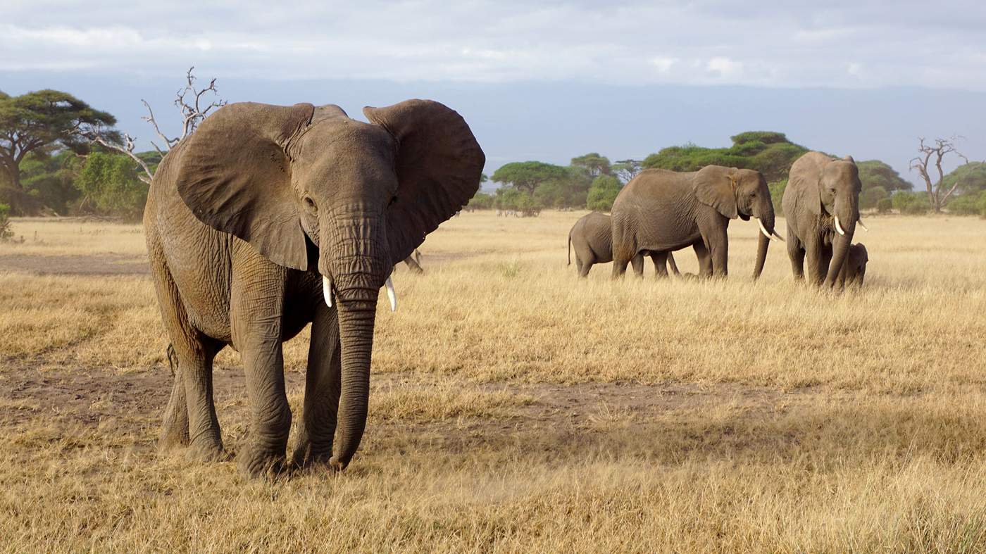
An Individual-Based Model of African elephant demography
In his PhD thesis, Severin Hauenstein developed a population model for African elephant. It describes survival and fecundity as a function of elephant size, rather than age (hence called an “integral projection model”, IPM). It thereby allows accommodating environmentally-driven variations in growth rates, e.g. less during droughts. Also, the carrying capacity, and hence the density-dependence of demographic rates, is integrated in this model. So far, this is so-called “mean-field approach”, in which no consideration is paid to variability between individuals: given their size, all individuals have the same model parameters.
An alternative approach to modelling population dynamics, “individual-based models” (a.k.a. agent-based models) allow representing variability among individuals. This is relevant only when the feature of interest, e.g. population size or population growth rate, is a non-linear function of the model parameters. That is the case in this demographic model. What is unclear is how much the representation of individual variability will affect model predictions.
The idea of this project is hence to re-implement the demographic model as an IBM, and compare the simulations with those of the original. One advantage of the IBM is that it is relatively easy to add further details and features. One disadvantage is that an IBM is much slower and hence more time-consuming to run repeatedly (This disadvantage should not be relevant for such a simple model).
Suitable as: MSc-project, requiring an interest in programming, preferably in python (or julia) or netlogo or C/C++ or, if need be, in R.
As BSc-project, various model improvements can be considered, e.g. integrating the currently separate calving model into the IPM, or a more GIS-related look-up functionality for extracting model parameters from the African Elephant Demographic Database.
Literature:
Boult, V. L., Quaife, T., Fishlock, V., Moss, C. J., Lee, P. C., & Sibly, R. M. (2018). Individual-based modelling of elephant population dynamics using remote sensing to estimate food availability. Ecological Modelling, 387, 187–195. https://doi.org/10.1016/j.ecolmodel.2018.09.010
Guestimating GHG break-even point for biomass gasification
Wood gas generation, using wood, manure, compost and like, produces CH4 under anaerobic conditions. Since renewable resources were used, biomass gas are considered sustainable etc. However, CH4 is a potent green-house gas, 84 times higher greenhouse warming potential than CO2 over 20 years ( https://en.wikipedia.org/wiki/Greenhouse_gas ) , and all biomass gasifiers leak. In industrial settings, leakage is under 5% ( https://www.umweltbundesamt.de/themen/biogasanlagen-muessen-sicherheiter-emissionsaermer ). In developing countries, particularly for self-made biomass generators and manual methan transport ( https://www.deutschlandfunk.de/mini-biogasanlagen-fuer-afrika-wirtschaftsfoerderung-statt.1773.de.html?dram:article_id=459738), such leakages can be expected to easily be in the 20-30%.
The aim of this project is to compute the break-even point of biomass gasification, given the global warming potential difference between CO2 and CH4. How much leakage is acceptable before causing more problems than solving them? The key point here is to (a) establish a transparent derivation of the balance; and (b) consider different time horizons of GHG activity of the two gases.
Suitable as: MSc project, in collaboration with Prof. Stefan Pauliuk (Industrial Ecology).
Fitting the elephant Integral Projection Model to observed data from Amboseli, Kenya
African elephant populations have been studied extensively. Local censuses date back to the 19th century and yet, historical estimates of the continental elephant population are scarce and uncertain. This project aims to estimate the population dynamics and spatial distribution of the African elephant from 1900 until today. Population size estimates can be derived from census reports and other published material. This project will be part of a larger demographic analysis of the continental African elephant population, which provides the opportunity to work alongside field and theoretical ecologists.
For his PhD, Severin Hauenstein has developed a population model, akin to, but more advanced than, a structured matrix population model. So far, this model is parameterised from literature data, yielding nice predictions for a population in Kenya.
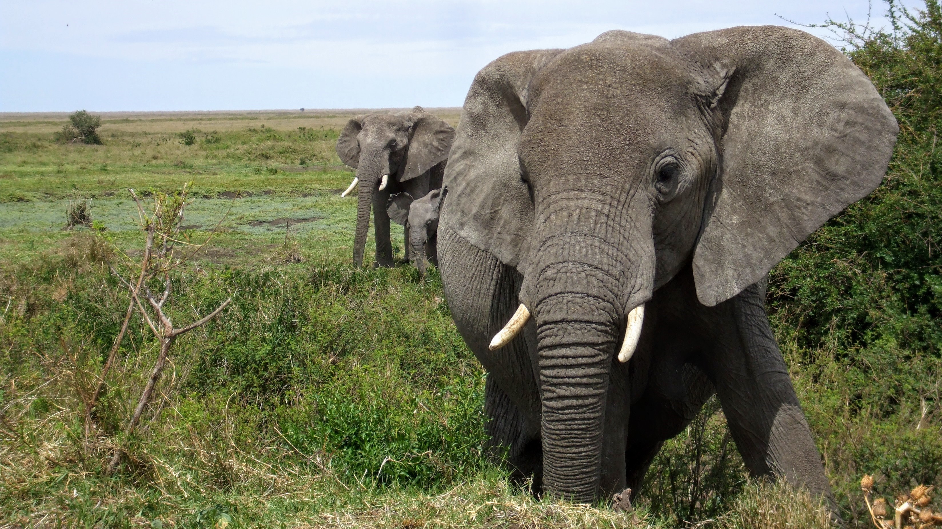
The next step, taken here, is to actually parameterise the model with the data of Amboseli, i.e. to fit the model to data. This requires a Bayesian model calibration approach, which is an intellectual hurdle, but also really cool. Apart from overall population size, the actual number of elephants in each age or size group will yield valuable information for the model parameters. The data are partially from elephant researchers in Africa, partially from the literautre. Data and model code are available, and tutorials for using Bayesian calibration are provided e.g. by R's BayesianTools package.
Suitable as: MSc project, requiring an interest in statistics and optimization.
Requirements: Willingness to engage in computer-intensive, statistical work.
Time: The project can start anytime.
Literature:
White, J. W., Nickols, K. J., Malone, D., Carr, M. H., Starr, R. M., Cordoleani, F., Baskett, M. L., Hastings, A., & Botsford, L. W. (2016). Fitting state-space integral projection models to size-structured time series data to estimate unknown parameters. Ecological Applications, 26(8), 2677–2694. https://doi.org/10.1002/eap.1398
Automatising statistical analyses
Why does every data set require the analyst to start over with all the things she has learned during her studies? Surely much of this can be automatised!
Apart from attempts to make human-readable output from statistical analyses, efforts to automatise even simple analyses have not made it onto the market. But some parts of a statistical analysis can surely be automatised, in a supportive way. For example, after fitting a model, model diagnostics should be relatively straight-forward to carry out and report automatically. Or a comparison of the fitted model with some hyperflexibel algorithm to see whether the model could be improved in principle. Or automatic proposals for the type of distribution to use, to deal with correlated predictors, or to plot main effects?
Here is your chance to have a go! In addition to the fun of inventing and implementing algorithms to automatically do something, you will realise why some things are not yet automatised.
This project has many potential dimensions. It could focus on traditional model diagnostics, or on automatised plotting, or on comparisons of GLMs with machine learning approaches to improve model structure, or ...
If you prefer, you can look at this project differently, in the context of "analyst degrees of freedom". The idea is that in any statistical analysis the analyst faces many decisions. Some are influential, others less so. As a consequence, the final p-values of an hypothesis test may be as reported, or may be distorted by the choices made. Implementing an "automatic statistician" as an interactive pipeline allows us to go through all combinations of decisions, in a factorial design, and evaluate which steps have large (bad) and which have small effects (good) on the correctness (nominal coverage) of the final p-value.
Requirements: Willingness to engage in R programming and abstract thinking. Frustration tolerance to error messages.
Time: The project can start anytime.
Identify underlying processes in multi-state environmental data using exploratory statistics and deep learning
In an environmental system, system states are causally linked in complex ways. For example, soil moisture affects sap flow and photosynthesis, but more rain does not mean more sap flow. Such non-linear interrelationships can be represented, in principle, by deep neural networks. Since the monitored data comprise drivers (radiation, rainfall) as well as responses (sap flow, soil moisture), and since the relevant processes act at potentially very different time scales (minutes to weeks), it is unclear (a) what the potential deep learning offers, and (b) how to efficiently construct such networks for maximal information gain. The aim would be to then inspect the represented relationships in order to improve our understanding of the system.
In a first step, data will be simulated using an ecosystem model (e.g. Landscape-DNDC or alike), so as to be sure that the linkages between processes and scales are known.
Two approaches seem to be interesting starting points: autoencoder (AE) and reservoir computing. AE is akin to a non-linear PCA and tries to reduce the dimensionality of the data by finding a simple, if non-linear, representation. It consists of an encoder and a decoder step, where the first leads to a latent description, while the latter links this back to the data. Copula?
Reservoir computing (e.g. echo state networks), in contrast, targets dynamic systems and work through representing the input (including lagged versions of the input) in a fixed but large set of possible interactions (the reservoir). Being “fixed” means here that weights are assigned randomly. Only the output (or rather the “readout” layer) is then linked to the response variable through linear regression.
Regrettably it is unclear, which approach seems particularly suitable for the problem at hand, and in how far the combined fitting of several system states actually infers and advantage of separate state-wise modelling (i.e. building a model for each Y separately using some ML algorithm).
Data are provided by the CAOS project from hydrology, which are multiple years of 12 system states in 40 sites, assessed at hourly intervals. (Also WSL data for only 1 year, or anything from EcoSense coming up.)
Process-integration into neural networks: using 3-PGN for PROFOUND
Neural network are all the rage. They require representative data, however, i.e. data that describe the underlying processes well. For many environmental systems, we have a rather good process understanding, particularly in forest growth, forest C-fluxes, but also in hydrology. In this case, it would be silly to ignore this knowledge when fitting a flashy neural network to observed data.
This project shall implement and compare different ways to integrate a process model into neural networks. The basic approach has been implemented and tested for C-fluxes in a boreal forest and a simply ecophysiological model. Now, the next step is to use a somewhat more flexible forest growth model, which in principle also represents mixed stands, N-dynamics and management (3-PGN).
Suitable as: MSc-project, requires interest in “deep learning” and python. Python code and data are available for the previous process model.
Contact: Carsten Dormann, carsten.dormann@biom.uni-freiburg.de
Literature: Willard, J., Jia, X., Xu, S., Steinbach, M., & Kumar, V. (2021). Integrating scientific knowledge with machine learning for engineering and environmental systems. ArXiv, 2003.04919 [physics, stat]. http://arxiv.org/abs/2003.04919
State-space model for tree-ring growth
Analysis of tree-ring width is a very standardised statistical approach, but it is neither intuitive, nor would it be what I would do based on how we teach GLMs and mixed-effect models.
Actually, this kind of data is surprisingly messy: they feature temporal autocorrelation, non-linear growth, depending on both age and previous year’s growth, and environmental /stand conditions around the trees.
The approach would thus be to 1. analyse some data in the way “everybody” does, and compare that to an incrementally more complicated 2. analysis more in line with non-linear state-space models. Ideally, and dependent on the skills and progress, data should be simulated with a specific growth model in mind, and then both approaches should be compared to whether they recover the parameters used.
Data will be available from international data bases, but also from the Forest Growth & Dendrochronology lab.
Literature:
Bowman, D. M. J. S., Brienen, R. J. W., Gloor, E., Phillips, O. L., & Prior, L. D. (2013). Detecting trends in tree growth: Not so simple. Trends in Plant Science, 18(1), 11–17. https://doi.org/10.1016/j.tplants.2012.08.005
Lundqvist, S.-O., Seifert, S., Grahn, T., Olsson, L., García-Gil, M. R., Karlsson, B., & Seifert, T. (2018). Age and weather effects on between and within ring variations of number, width and coarseness of tracheids and radial growth of young Norway spruce. European Journal of Forest Research, 137(5), 719–743. https://doi.org/10.1007/s10342-018-1136-x
Schofield, M. R., Barker, R. J., Gelman, A., Cook, E. R., & Briffa, K. R. (2016). A model-based approach to climate reconstruction using tree-ring data. Journal of the American Statistical Association, 111(513), 93–106. https://doi.org/10.1080/01621459.2015.1110524
Zhao, S., Pederson, N., D’Orangeville, L., HilleRisLambers, J., Boose, E., Penone, C., Bauer, B., Jiang, Y., & Manzanedo, R. D. (2019). The International Tree-Ring Data Bank (ITRDB) revisited: Data availability and global ecological representativity. Journal of Biogeography, 46(2), 355–368. https://doi.org/10.1111/jbi.13488
Post-selection inference for regression: (how) does it work?
One of the better-kept secrets in applied statistics is that model selection destroys P-values. That means, if we start with a regression model with many predictors and stepwisely remove all those deemed irrelevant for the model (e.g. based on the AIC), we introduce a bias in the resulting final model, its estimates, their standard error and hence their P-values.
There are a few studies trying to save the resulting model from misinterpretation. They aim at producing correct P-values despite model selection. These studies fly under the name of “post-selection inference”. Does it work? How does it work? And why does it work (if it does)? This thesis will use simulated data to first demonstrate the problem of selection for P-values in regression, then employ post-selection inference approaches to fix them. It will, hopefully, result in a tutorial useful for others in this situation.
Literature:
Kuchibhotla, A. K., Kolassa, J. E., & Kuffner, T. A. (2022). Post-selection inference. Annual Review of Statistics and Its Application, 9(1), 505–527. https://doi.org/10.1146/annurev-statistics-100421-044639
Lee, J. D., Sun, D. L., Sun, Y., & Taylor, J. E. (2016). Exact post-selection inference, with application to the lasso. The Annals of Statistics, 44(3), 907–927. https://doi.org/10.1214/15-AOS1371
What do we actually know in ecology? Ask ChatGPT!
Ecology textbooks are thick tombs, not because we know so much about how ecological system work, but because ecology is a science taught be telling anecdotes and interesting case studies. Applied ecology then resorts to doing the same experiments and analyses again for the specific question at hand, indicating that we do not really trust ecological principles. Really, what do we know?
Since ecologists cannot possibly keep up with the thousands of paper published every year, they read “only” the material relevant for their own research or system, and the “tabloid” publications (in Nature and Science). How distorted is the picture that emerges from such selective reading?
Large-Language Models such as GPT cannot reason, but they are (apparently) very good in extracting information. They offer, for the first time in history, a way to summarise vast amounts of text in what seems to be a meaningful way. Thus, they can be used to compare the ecological knowledge presented in Nature/Science with that in classical ecology textbooks. This is a rather experimental thesis, as it is unclear how well LLMs can actually do the work in question. One starting point is to investigate species subfields in ecology, such as “assembly rules” or “non-equilibrium coexistence” or “effects of biodiversity”. Once a pipeline has been established, a tutorial could help others to do the same for their field.
See here for some initial ideas on how to proceed:
https://platform.openai.com/docs/guides/fine-tuning/create-a-fine-tuned-model
https://schwitzsplinters.blogspot.com/2022/07/results-computerized-philosopher-can.html
Identifying subpopulation structures of wide-spread species from distribution data using spatially-variable regression. For wide-spread species such as wolf, birch and tuna, local adaptation to rather different climatic and environmental conditions has led to recognisable subspecies. Current analyses of species distributions, which aim at describing a species’ environmental preferences or “niche”, treat a species as if it had a single, constant niche. Using a more flexible approach, where the habitat preferences are allowed to change in space, may be a way to both better represent and even detect subpopulations within species.
This project will analyse a range of different species (and possibly genera) to explore whether this spatially-variable coefficient approach is an improvement over spatially constant models, and whether subpopulations identified align with our knowledge of the genetic substructure for that species.
Literature:
Doser, J. W., Kéry, M., Saunders, S. P., Finley, A. O., Bateman, B. L., Grand, J., Reault, S., Weed, A. S., & Zipkin, E. F. (2024). Guidelines for the use of spatially varying coefficients in species distribution models. Global Ecology and Biogeography, 33(4), e13814. https://doi.org/10.1111/geb.13814
Osborne, P. E., Foody, G. M., & Suárez-Seoane, S. (2007). Non-stationarity and local approaches to modelling the distributions of wildlife. Diversity and Distributions, 13, 313–323.
Thorson, J. T., Barnes, C. L., Friedman, S. T., Morano, J. L., & Siple, M. C. (2023). Spatially varying coefficients can improve parsimony and descriptive power for species distribution models. Ecography, 2023(5), e06510. https://doi.org/10.1111/ecog.06510
Dynamic energy budgets for ungulate: adding movement
Topic: In a very reductionist, but highly useful, view of organisms as physical machines, each individual has to maintain a positive energy balance. In an approach called "dynamic energy budget", Bas Kooijman
It is implemented in software (e.g. R's NicheMapR::deb mrke.github.io/models/Dynamic-Energy-Budget-Models) and can thus be relatively simple be used to describe energy demand and net positive energy balances for a species at any place on the (terrestrial) world. What is missing, so far, is the additional costs incurred by movement. These are so far included in the basic metabolic rates of moving organisms, but that seems insufficient for migratory species (think: caribou, wildebeest and alike).
The aim of this project is to first establish the DEB approach for a migratory or at least widely moving ungulate species and then add the movement costs, based on allometric scaling (i.e. the general power-law relationship between movement cost and body size). A comparison of suitable range sizes before and after adding the movement module provide an assessment of the potential relevance of this term. (For very few species will we be able to validate the correctness of such an approach, as it requires measurement of metabolic costs in the field, and during different stages of movement; difficult, but not impossible.)
Suitable as: MSc project.
Requirements: Ability and willingness to think conceptually about energy consumption and metabolics. Familiarity with running R. Affinity to mathematical equations (those that describe the energy budget).
Time: Start anytime
Predicting x from y: methods and examples for inverse regressions
Particularly in ecotoxicology, but also in other fields of science, do we want to “invert” a fitted curve. That is, we want to predict x from y. Imagine, for example, that we analyse the effect of drought on tree mortality. Then we may want to ask the inverse question: at what level of drought do we see a 50% die-off? The challenge of this inversion is that we cannot simply invert the axes and do a new regression (of x against y): our error is on the response, and hence regression techniques are not equipped to deal with error on the x-axis. The BSc thesis reviews and implements different approaches to estimate x from y, given a fitted regression, and the error bars for the resulting predicted x-values. A practical implication is provided by a forest restoration project, in which we want to estimate after how many years the plant, ant and bird communities are 90% similar to the original primary forest again. The resulting how-to guide will go from simple, linear cases to more complicated non-linear functions.
Literature:
Halperin, M. (1970). On inverse estimation in linear regression. Technometrics, 12(4), 727–736. https://doi.org/10.1080/00401706.1970.10488723
Lavagnini, I., Badocco, D., Pastore, P., & Magno, F. (2011). Theil–Sen nonparametric regression technique on univariate calibration, inverse regression and detection limits. Talanta, 87, 180–188. https://doi.org/10.1016/j.talanta.2011.09.059
Lavagnini, I., & Magno, F. (2007). A statistical overview on univariate calibration, inverse regression, and detection limits: Application to gas chromatography/mass spectrometry technique. Mass Spectrometry Reviews, 26(1), 1–18. https://doi.org/10.1002/mas.20100
Ritz, C., Baty, F., Streibig, J. C., & Gerhard, D. (2015). Dose-response analysis using R. PLoS ONE, 10(12), e0146021.
https://doi.org/10.1371/journal.pone.0146021
How important is recruitment for forests? From simple to complex answers
A forest tree lives for decades, if not centuries (depending on where in the world this forest is found). During this time, it may produce thousands to millions of seeds, most of which are eaten, infected by molds or fall onto unsuitable ground. But in principle it only requires a single seed to germinate and grow to eventually replace the parent tree. The situation is complicated, in the tropics at least, by an intense competition for the few gap that become available as an old tree falls; having more seeds in the lottery increases the chance of recruiting successfully. However, that is “only” the evolutionary answer to why trees produce so many more seeds than required for self-replacement. It does not answer the question whether the forest would look different if all trees would produce, say, only 10% of the current number of seeds.
Forest researchers do not live as long as their study objects, and funded projects are even shorter. We may observe reduced recruitment for a spell of five dry years, or intensive mould for several fruiting periods, but does that matter for the forest? Without clever modelling, we cannot get an intuition of how important recruitment of forest trees is for forest dynamics.
This project aims at providing different modelling entries to the problem. It will proceed from back-of-the-envelop calculations to aggregated and then individual-based forest growth models to answer the same question: what is the effect of halving, or doubling, recruitment rates for two very different forest systems (one tropical, one temperate)?
The literature is somewhat sparse on this topic. While there are thousands of papers on germination limitation and factors that affect recruitment, it is not easy to find publications with a several-hundred-years-perspective. Forest growth models often, but not always, have a recruitment module (e.g. Formind, and the entire class of forest gap models).
Literature:
Bowman, D. M. J. S., Brienen, R. J. W., Gloor, E., Phillips, O. L., & Prior, L. D. (2013). Detecting trends in tree growth: Not so simple. Trends in Plant Science, 18(1), 11–17. https://doi.org/10.1016/j.tplants.2012.08.005
Lundqvist, S.-O., Seifert, S., Grahn, T., Olsson, L., García-Gil, M. R., Karlsson, B., & Seifert, T. (2018). Age and weather effects on between and within ring variations of number, width and coarseness of tracheids and radial growth of young Norway spruce. European Journal of Forest Research, 137(5), 719–743. https://doi.org/10.1007/s10342-018-1136-x
Schofield, M. R., Barker, R. J., Gelman, A., Cook, E. R., & Briffa, K. R. (2016). A model-based approach to climate reconstruction using tree-ring data. Journal of the American Statistical Association, 111(513), 93–106. https://doi.org/10.1080/01621459.2015.1110524
Zhao, S., Pederson, N., D’Orangeville, L., HilleRisLambers, J., Boose, E., Penone, C., Bauer, B., Jiang, Y., & Manzanedo, R. D. (2019). The International Tree-Ring Data Bank (ITRDB) revisited: Data availability and global ecological representativity. Journal of Biogeography, 46(2), 355–368. https://doi.org/10.1111/jbi.13488
State-space model of tree growth
Statistical representation of tree (ring) growth is not trivial. The main problem is that each observed growth increment (a tree ring) is a function of last year’s growth (and possibly several previous years, too). Hence, the model needs to represent the state of the tree several years back in time in order to predict its current growth. Such lagged models are further complicated by the fact that what we observe, the tree ring, does not directly represent its function some years ago. Thus, there is a discrepancy between observation and the true but unobserved (“latent”) state relevant for tree growth.
Two general approaches are feasible in this situation, depending on whether all system states are considered endogenous or not. If so, vector autoregressive models (VAR) represent a nice and relatively simple solution. If not, and that is typically the case for trees growing in dependence of weather and management, we require a state-space representation (SSM).
This project will compare a SSM with a VAR for the growth of spruce from different sites in the Black Forest.
Literature:
Bowman, D. M. J. S., Brienen, R. J. W., Gloor, E., Phillips, O. L., & Prior, L. D. (2013). Detecting trends in tree growth: Not so simple. Trends in Plant Science, 18(1), 11–17. https://doi.org/10.1016/j.tplants.2012.08.005
Clark, J. S., Wolosin, M., Dietze, M., IbáÑez, I., LaDeau, S., Welsh, M., & Kloeppel, B. (2007). Tree growth inference and prediction from diameter censuses and ring widths. Ecological Applications, 17(7), 1942–1953. https://doi.org/10.1890/06-1039.1
Dietze, M. C., Wolosin, M. S., & Clark, J. S. (2008). Capturing diversity and interspecific variability in allometries: A hierarchical approach. Forest Ecology and Management, 256(11), 1939–1948. https://doi.org/10.1016/j.foreco.2008.07.034
Lundqvist, S.-O., Seifert, S., Grahn, T., Olsson, L., García-Gil, M. R., Karlsson, B., & Seifert, T. (2018). Age and weather effects on between and within ring variations of number, width and coarseness of tracheids and radial growth of young Norway spruce. European Journal of Forest Research, 137(5), 719–743. https://doi.org/10.1007/s10342-018-1136-x
Schofield, M. R., Barker, R. J., Gelman, A., Cook, E. R., & Briffa, K. R. (2016). A model-based approach to climate reconstruction using tree-ring data. Journal of the American Statistical Association, 111(513), 93–106. https://doi.org/10.1080/01621459.2015.1110524
Zhao, S., Pederson, N., D’Orangeville, L., HilleRisLambers, J., Boose, E., Penone, C., Bauer, B., Jiang, Y., & Manzanedo, R. D. (2019). The International Tree-Ring Data Bank (ITRDB) revisited: Data availability and global ecological representativity. Journal of Biogeography, 46(2), 355–368. https://doi.org/10.1111/jbi.13488
Variable selection prevents scientific progress
In multiple regression, it is common to exclude one of a pair of highly correlated variables. As a consequence, the remaining variable is now a representative for both original variables. However, in the publications people typically interpret only the remaining predictor. Attributing the effect (in a meta-analysis) to the selected variable is thus optimistic and biased – making meta-analyses of the results of model selection worthless.
This project will show, through some simple proof-of-principle simulation, that this point is correct. Using a representative sample of studies from the ecological literature on biodiversity, it will then quantify the problem: which proportion of studies did it wrong, how many remain, and how much reported effort was thus wasted for synthesising science?
Growth responses of European Beech to drought - reanalysed
Re-analyse the paper of Martinez del Castillo et al. (2022) using a spatially variable coefficient model. First only on a single section of growth data, then possibly including all growth data in one go. The aim is to (a) identify ecotypic variation in growth, and (b) to simply map growth variation more flexibly than was done in that paper.
This is a BSc-project for a person with interests in getting familiar with some more advanced-yet-traditional statistical approaches. For an MSc-project, this links additionally to previous work and will include a review of the statistical approach and its validation.
Literature:
Martinez del Castillo, E., Zang, C. S., Buras, A., … de Luis, M. (2022). Climate-change-driven growth decline of European beech forests. Communications Biology, 5(1), 1–9. https://doi.org/10.1038/s42003-022-03107-3
Individual-based models vs mean-field approach: what do we need?
Topic: In ecology and sociology, the huge variability in behaviour and the large variability in any trait of relevance among individuals has led to a strong push for so-called "individual-based" models, aka "agent-based models". These represent individuals, with fixed traits, but large variation among individuals. Such IBM/ABMs contrast with traditional, "theoretical" models, which are referred to as "mean-field approaches" (MFA).
It can be easily shown, for hypothetical situations, that IBM and MFAs may differ substantially in population dynamics. But does this potential difference actually matter in real systems?
Methods: Literature review of all studies comparing IBM and MFA. In google scholar, "("individual-based model" or "agent-based model") AND "mean field"" yields just over 200 papers, most probably irrelevant.
Suitable as: BSc or MSc thesis project
Time: A start is possible at any time.
Requirements: Interests in rather abstract system descriptions and model behaviour; meta-analysis.
Extinction scenarios for interaction networks
One interest in interaction networks in ecology is due to the idea that such network structure actually matters for the functioning of the system, or the robustness to change. Simulating extinctions from a network is thus a frequently used way to assess extinction consequences, even though the assumptions behind such simulations are ecologically not realistic. For example, one would expect a pollinator to change its preferences when the preferred flower species is absent, rather than simply go extinct.
Extinction sequences can thus be based on different assumptions: no adaptation, replacement by the most similar flower type, etc. Simulating such different extinction scenarios and quantifying the network robustness will show how different they actually are, and whether it is important to consider shifts in interactions.
Currently, only one study looked at such shifts in preferences, a.k.a. “rewiring” (Vizentin-Bugoni et al. 2019). It shows that there is indeed an effect, but it fails to identify the causes: is it due to abundance distributions, or to the way traits are distributed across species? Why does combining different traits have no effect? Such questions can only be addressed by simulating interaction networks and running them through different types of rewiring scenarios. That is exactly the idea for this project.
Suitable as: MSc project, requiring comfortable use of R and willingness to think abstractly about networks, without any obvious non-academic application.
Literature: Vizentin‐Bugoni, J., Debastiani, V. J., Bastazini, V. A. G., Maruyama, P. K., & Sperry, J. H. (2019). Including rewiring in the estimation of the robustness of mutualistic networks. Methods in Ecology and Evolution, in press. https://doi.org/10.1111/2041-210X.13306
Confidence intervals for subsampled regression models
Sometimes a data set is so big that you can't process it completely with one method (e.g. a spatial model that can't handle over 5000 data points). If we then takes a subsample, about 5000 points of the maybe 1 million data points in total, then we totally overestimate the error bar of the regression. Is there no way to correct this? Yes, you can. There is a nice statistical theory about this in the book "Subsampling" from 1999, but you have to estimate a parameter for it from the data (by trying subsamples of different sizes). According to my survey, no one has ever done this, at least not in ecology, but I think it is very practical, precisely because there are often models that we can only run on a subsample of the data.
The aim of the work would be to get this approach working on the basis of simulated data and to present it for a large data set (from a Science paper) (here a spatial GLS is to be approximated for >600000 data points). Pretty cool, probably a bit of fiddling, but in my opinion easy to complete, including a manuscript. A first step would be to review the literature and confirm the absence of this idea from it, as the opposite step has been taken for other purposes (“data cloning”).
Suitable as: Both as BSc- or MSc project, requiring some interest in statistical analysis and R-coding. Allergy to mathematical equations would be problematic, even though the majority of the work would be demonstration-by-simulation, not through maths.
Literature:
Absent from the ecological literature, but for maths see, e.g., Wang, H., Zhu, R., & Ma, P. (2018). Optimal subsampling for large sample logistic regression. Journal of the American Statistical Association, 113(522), 829–844. https://doi.org/10.1080/01621459.2017.1292914
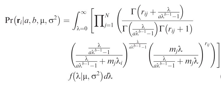
Unified sampling model for abundance of species in communities: fitting an ugly likelihood using MCMC [R programming; community data analysis]
How many individuals would we expect a species to have in a local community? That may sound like a strange question, but then we do observe that most species are rare, only some are very common. So there is a pattern! Since several years, Sean Connolly has attempted to find a statistical distribution that describes how many individuals to expect for each species of a community across samples from many sites. The result is a very ugly distribution, but it has the potential to be enormously useful! Alongside the equation, Connolly et al. (2017) also provide a function to fit this ugly distribution, but it only works reliably for large data set (many species, many individuals, many sites), which severely limits its usefulness.
This project attempt to use an MCMC-fitting algorithm (of the many existing ones) to estimate the parameters of the ugly equation in a more robust way. Also, we can expect that the parameters of this distribution are dependent on the environment, which is currently not implemented in Connolly et al.'s functions. This way, one could use the ugly equation to estimate the effect of, say, landscape structure on abundances of birds or spiders in a statistically satisfying way: using the information of all species, rather than only the number of species or a diversity index.
Methods: R programming: Develop/adopt MCMC-sampler to fitting the ugly equation (→).
Analysis: Apply to one or more community data along a landscape structure gradient.
Requirements: Basic mathematics: The ugly function features all sorts of mathematical niceties, which at least require tolerance to formulae.
Time: The project can start anytime. Suitable as MSc project.
References:
Connolly, S.R., Hughes, T.P. & Bellwood, D.R. (2017) A unified model explains commonness and rarity on coral reefs. Ecology Letters, 20, 477–486.
Effect of close-to-nature recreational activities on wildlife behaviour, contrasting hunting and non-hunting zones [Literature review]
National parks serve the dual purpose of conservation and recreation. However, park visitors may affect wildlife behaviour, such as day-night-activity patterns, habitat use or uphill migration. How animals respond to visitors seems to depend hugely on the type of activity (hiking or paragliding, mountain-biking or cross-country skiing), as well as on the individual animal's experience with humans. Large north American national parks (such as Yellowstone or Banff) host almost tame ungulates, while similar species in most European parks are very timid. This project shall test the hypothesis that it is the hunting history that determines how animals respond to human visitors. After several decades of full protection from hunting, we expect animals to become much less shy. This project shall review existing studies and reports from around the world, contrasting wildlife behaviour in hunting and non-hunting zones. Depending on the material available, the focus would narrow down to ungulates, predators and large birds, and to the northern hemisphere.
Methods
Literature review. First a scoping study will identify the number of studies available. Then species and regions will be selected, and studies with clear

hunting on/off-regimes identified. Key target behaviours are flight-initiation-distance and day/night activity budgets.
Time: The project can start anytime. Suitable MSc project.
Requirements: Willingness to wade through substantial and scattered publications.
Soya growing area of the future - model-based prediction of the suitability for cultivation of soybeans in Climate Change
The cultivation of soybeans in Germany reached an all-time high of around 33,000 ha in 2020 Acreage. According to data from the Deutsches Sojaförderring e.V.1, this corresponds to only about 2% of the annual demand in soybean in Germany. On a national as well as European level, climatic changes are expected to increase cover by around 50% through domestic production in the medium term (Roßberg and Recknagel 2017; Guilpart et al. 2020).
An increase in the soya cultivation area has in addition to numerous positive ecological aspects (e.g. Nemecek et al. 2008) direct political relevance (see e.g. the European soya Explanation2). For long-term use of the cultivation potential is it is necessary to identify future favoured areas in advance and to establish appropriate agricultural structures. In the course of climate change, the opposite effects can appear. While an elevated temperature in the growing season lead to a significant increase in cultivability (Guilpart et al. 2020), at the same time there is an increased risk of summer drought (Spinoni et al. 2017; Spinoni et al. 2018). In particular drought stress from the time of flowering significantly reduces the yield (Meckel et al. 1984; Frederick et al. 2001). This effect can be seen already at the regional level in the contract farming data from Taifun-Tofu GmbH. Despite this conflict, current models lack critical parameters such as precipitation or water retention capacity of soils (Guilpart et al. 2020).
The advertised thesis is intended to close this gap:
- Evaluation of the map of the current suitability for cultivation of soybean in Germany (figure above) under the requirements of the ability to predict climate change
- Modelling the shift in cultivation suitability under different climate projections on the basis the map of suitability for cultivation of soyabeans
- Analysis of the effects of increased summer drought on regional cultivation worthiness
The Deutsche version and full literature list for this advert can be found here.
Suitable as: BSc or MSc thesis project
Contact: Stefan Paul < s.paul@taifun-tofu.de>
Reference:
1https://www.sojafoerderring.de/
2https://www.donausoja.org/fileadmin/user_upload/Activity/Media/European_Soya_signed_declaration.pdf
Literature:
Frederick, James R.; Camp, Carl R.; Bauer, Philip J. (2001): Drought‐Stress Effects on Branch and Mainstem Seed Yield and Yield Components of Determinate Soybean. In: Crop Sci. 41 (3), S. 759–763. DOI: 10.2135/cropsci2001.413759x.
Guilpart, Nicolas; Toshichika, Iizumi; David, Makowski (2020): Data-driven yield projections suggest large opportunities to improve Europe’s soybean self-sufficiency under climate change. In: bioRxiv, 2020.10.08.331496. DOI: 10.1101/2020.10.08.331496.
Extension of the map of suitability for cultivation of soya beans
Despite political declarations of intent (e.g. by the European Soya Declaration1), the European Union is strongly dependent on international soya imports (Fig. 1, Kezeya et al. 2020).
On the way to a meaningful nutritional provisioning at national, as well as at the European level, in the medium term around 50% of the demand could be covered from domestic production (Roßberg and Recknagel 2017; Guilpart et al. 2020). In addition to plant cultivation, an increase in the soya cultivation area also has numerous positive ecological aspects (e.g. Nemecek et al. 2008).
For an expansion of the soya cultivation it is important to identify cultivation suitability of undeveloped areas in advance. For this purpose, region-specific field tests, as well as location factors-based ex-ante evaluations (Rossiter 1996) are used. Newer models are also used for predictions under different climate scenarios (e.g. Daccache et al. 2012) or to consider economic approaches in the modelling of cultivation suitability (Marraccini et al. 2020).
In Germany, the "map of growing suitability of soyabeans” has established as a useful tool for cultivation advice (Fig. 2, Roßberg and Recknagel 2017). Cultivation suitability for soybeans is determined by means of readily available data such as mean land value figures, total precipitation, global radiation, as well as the CHU heat sums are calculated. Despite the simple concept the map shows a high overlap with the data of the contract cultivation of the Taifun-Tofu GmbH. However, the limitation to the area of the Federal Republic of Germany is very restrictive. European approaches are developed but often remain limited to specific regions (Marraccini et al. 2020) or a small set of climatic parameters (Guilpart et al. 2020).
The advertised work starts at this point and includes the following subject areas:
- Analysis of existing data for Central and Western Europe
- If necessary, adapt the model of the "map of Germany on the suitability of soybeans to be cultivated", depending on data availability and quality
- Calculation of cultivation suitability for available regions / countries
- Comparison of the model-based cultivation suitability with current cultivation areas
The Deutsche version and full literature list for this advert can be found here.
Suitable as: BSc or MSc thesis project
Contact: Stefan Paul < s.paul@taifun-tofu.de>
Reference:
1https://www.donausoja.org/fileadmin/user_upload/Activity/Media/European_Soya_signed_declaration.pdf
Literature:
Daccache, Andre; KEAY, C .; Jones, Robert JA; WEATHERHEAD, EK; STALHAM, MA; Knox, Jerry W. (2012): Climate change and land suitability for potato production in England and Wales: impacts and adaptation. In: J. Agric. Sci . 150 (2), pp. 161-177.
Guilpart, Nicolas; Toshichika, Iizumi; David, Makowski (2020): Data-driven yield projections suggest large opportunities to improve Europe's soybean self-sufficiency under climate change. In: bioRxiv , 2020.10.08.331496. DOI: 10.1101 / 2020.10.08.331496.